Rendering Layered Materials
by Markus Worchel and Alexander Lelidis
For the the computer graphics seminar 2015-16 we decided to implement the paper A Comprehensive Framework for Rendering Layered Materials from Jakob Wenzel [1]. The paper presents a new method for rendering material consisting of multiple layers by precomputing the reflection model. The technique supports arbitrary composition of materials and correctly accounts for multiple scattering within and between layers. In terms of a rendering system the models are efficient to evaluate. By exploiting the concepts of sparse matrix representation, the precomputed values can be stored space efficently, even for high glossy materials, and be reused for different scenes.
Overview
In this section we are going to give an overview of the basic theory. At first we want to point out, that in the scope of the seminar we focused on the preprocessing part of the model, which includes representing of layered materials as scattering tensors. For the final rendering we used PBRT V3 framework [3].
Because every layer represents either a medium or a boundary and we want to be able to store the result, we need to discretize the phase and BSD functions. In the following part we are only going to look at BSDFs, because phase functions can be handled analogous. A BSDF is a function of 4 parameters , which models the illumination behavior of a material given in and outgoing direction. $$ \mathbb{R}^4 \to \mathbb{R} : f(\mu_i, \phi_i, \mu_o, \phi_o) $$ The directions are encoded as the cosine of the elevation angle \( \mu \) and the azimuth angle \( \phi \). Using isotropy assumptions, we are able to reduce the function to a function of 3 parameters. $$ \mathbb{R}^3 \to \mathbb{R} : f(\mu_i, \mu_o, \phi_d) $$ where \( \phi_d = |\phi_i - \phi_o| \). In order to further reduce the dimension of the domain, we sample \( \mu \) from \( [-1, 1] \). Therefore we use the GaussLobatto points. Now the BSDF only depends on one parameter. $$ \mathbb{R} \to \mathbb{R} : f_{\mu_i, \mu_o}(\phi_d) $$ The last step to remove the remaining parameter by projecting the BSDF function into fourier space, by representing it with even fourier basis approximating it with k fourier orders. $$ f_{\mu_i, \mu_o}(\phi_d) = \sum\limits_{l = 0}^{k} c_{\mu_i, \mu_o}(l) \cos(l \phi_d) $$ where c(l) denotes the l-th Fourier coefficient of f as a function of azimuth for fixed \(\mu_i\) and \(\mu_o\).
The main challange is to find a fourier representation of a resonable BSDF model. In the paper they choose the microfacet model by Walter et al. [2]. This model consists of a reflection and a transmission term. $$ f(\mu_i, \phi_i, \mu_o, \phi_o) = f_r(\mu_i, \mu_o, \phi_i - \phi_o) + f_t(\mu_i, \mu_o, \phi_i - \phi_o) $$ The reflection term \(f_r\) is defined as $$ f_r(\mu_i, \mu_o, \phi_i - \phi_o) = \frac{F(\mu_h)D(\mu_h)G(\mu_i, \mu_o)}{4|\mu_i\mu_o|} $$ where F specifies the Fresnel reflectance, D is the Beckmann distribution, G is a shadowing-masking term, and \(\mu_h\) denotes the cosine of the angle between the normal and the half-direction vector of the incident and outgoing directions. However, they were not able to find an analytic transformation for this model due to the significant complexity, for that reason they are forced to turn to numerical integration.
The final discretized function is represented as a tensor, for every fourier level we have a quadratic scattering matrix, which contains the coefficents of this level. The size depends on the amount of samples in \(\mu\). For a level l we get the following scattering matrix: $$ \left[ \begin{array}{c|c} T_l^{tb} & R_l^b \\ \hline R_l^t & T_l^{bt} \end{array} \right] = \pi (1 + \delta_{0l}) \left[ \begin{array}{c|c} F_l^{tb} & F_l^b \\ \hline F_l^t & F_l^{bt} \end{array} \right] W \overline{M} $$ where $$ F_l := (c_{\mu_i, \mu_o}(l))_{ij} \in \mathbb{R}^{n \times n} $$ $$ W := (\delta_{ij}w_i)_{ij} \in \mathbb{R}^{n \times n} $$ $$ \overline{M} := (\delta_{ij}|\mu_i|)_{ij} \in \mathbb{R}^{n \times n} $$ M are the samples from the GaussLobatto method and the W contains the corresponding weights. The result is a block matrix where R represents the reflective part and the T the transmissive of the current BSDF on the given fourier level.
The scattering is now a discrete approximation of the BSDF reflection and transmission behavior. Since the goal was to rrepresent layered materials, we are going to stack two materials by combining the tensor of both materials. For this step they use the adding equation: $$ \overline{R}^t = R^t_1 + T^{bt}_1(I - R_2^t R_1^b)^{-1} R_2^t T_1^{tb} $$ $$ \overline{R}^b = R^b_2 + T^{tb}_2(I - R_1^b R_2^t)^{-1} R_1^b T_2^{bt} $$ $$ \overline{T}^{tb} = T_2^{tb}(I - R_1^b R_2^t)^{-1} T_1^{tb} $$ $$ \overline{T}^{bt} = T_1^{bt}(I - R_2^t R_1^b)^{-1} T_2^{bt} $$ This results in new scattering matrix for each level with represents the combined material.
Implementation
For our implementation we decided to use the script language python 3.4, together with the packages numpy, scipy and matplot lib for plotting the matices. For the data exchange between our implementation and the render we used the format proposed by the paper, which is also supported by PBRT V3. The following code snippet shows how to create layers in our implementation and how to combine them to a new layered material.
albedo = 0.5
eta_top = 1.5
alpha  = 0.02  # Beckmann roughness
eta_bot = get_rgb(gold)

alpha_top = 0.1  # Beckmann roughness of top layer (coating)
alpha_bot = 0.1  # Beckmann roughness of bottom layer (gold)

n = 196
m = 267
mu, w = gaussLobatto(n)

# 1. Creating coating layer
coating = layer(mu, w, m)
coating.setMicrofacet(eta_top, alpha_top)

output = []
for channel in range(3):
    # Construct gold bottom layer for each channel
    # 2. Creating metal layer
    l = layer(mu, w, m)
    l.setMicrofacet(eta_bot[channel], alpha_bot)

    # Apply coating
    # 3. Applying coating..
    output.append(layer.addToTop(coating, l))
Results
In this section we are going to describe our results. The start with the comparsion of the BSDF/ phase functions to their fourier approximation. Afterwards be compare for each level our scattering matrix with the scattering obtained by using the reference implementation. Finally we visually compare our results of rendering layered materials with reference images from the paper.
Fourier approximation
BSDF fourier
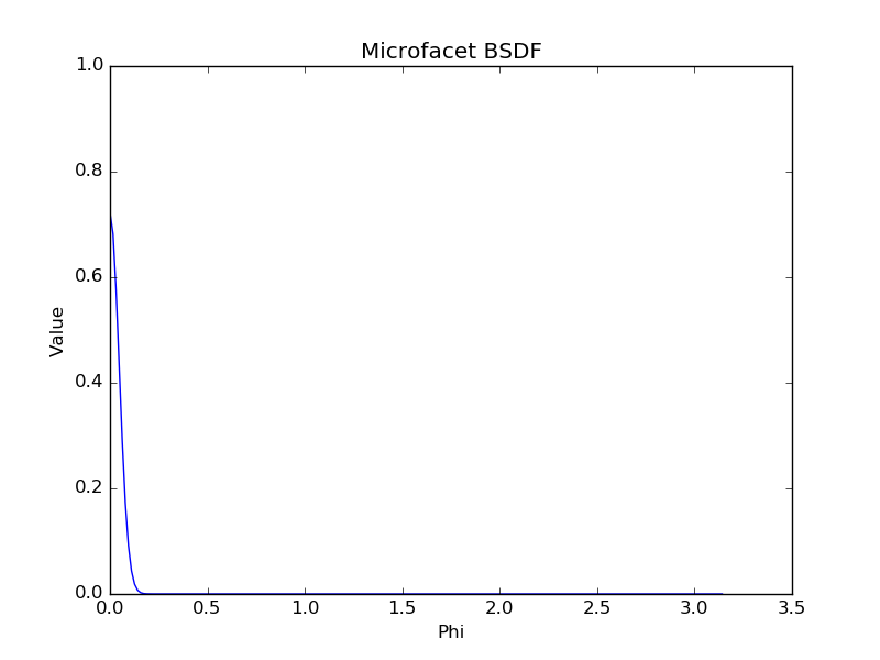
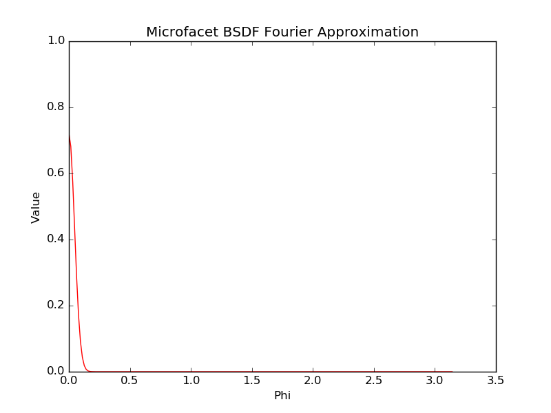
Comparison of original microfacet BSDF and our reconstruction from 100 fourier coefficents. We used the following values: \(\mu_i = 0.5\), \(\mu_o = -0.6\), \(\alpha = 0.05\) and \(\eta = 1.1\)
BSDF fourier error

This plot shows the absolute error between the approximation and the original BSDF with increasing number of fourier coefficents. We use the same parameters as before.
Scattering matrices
Diffuse

Scattering matrix of first fourier level of a diffuse layer with albedo 0.8
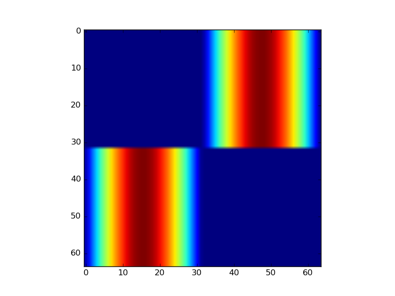
Microfacet
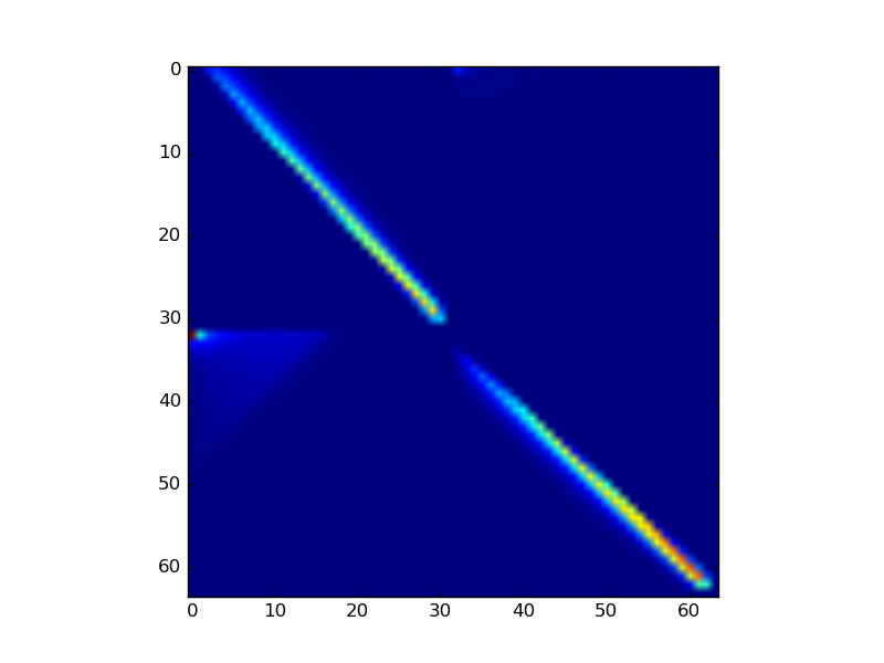

Comparison between our and the the reference implementation of a microfacet BSDF scattering matrix of fourier level 3 representing a rough dielectric. We used 64 samples in \(\mu\), \(\eta = 1.1\) and \(\alpha = 0.6\).
Adding equation

This image compares for each RGB channel the scattering materices as a result of the adding equations. The matrices represent a combined material, composed of gold and coating. The animation cycle trough the first 30 fourier levels.
Renderings
Diffuse

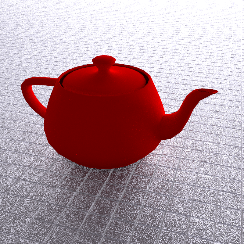
Comparison of our rendering and reference rendering of a diffuse material on a teapot represented by a single fourier level scattering matrix. We're using 256 samples per pixel and 128 samples in \(\mu\).
Rough dielectric,Silver and copper
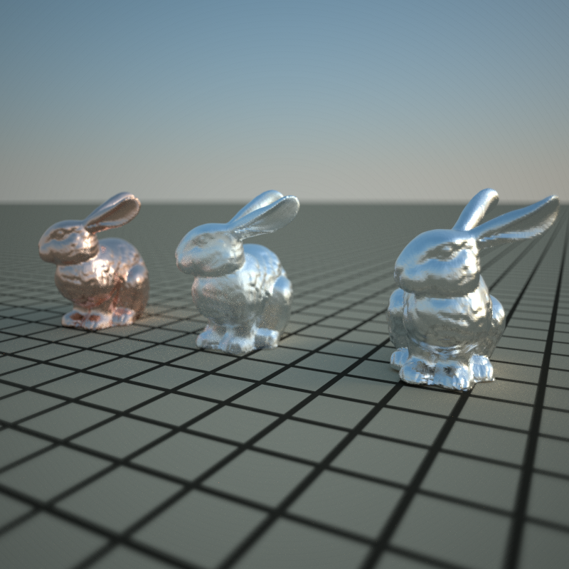

Rendering of three teapots, one silver metal, one copper and one rough dielectric. The image shows a comparison of our rendering and the reference rendering. The materials were represented by scattering matrices with multiple fourier orders (TODO: number of fourier orders per material?!) and XXX samples in \(\mu\).
Coated Gold (Dragons 2 types coated and not coated gold)
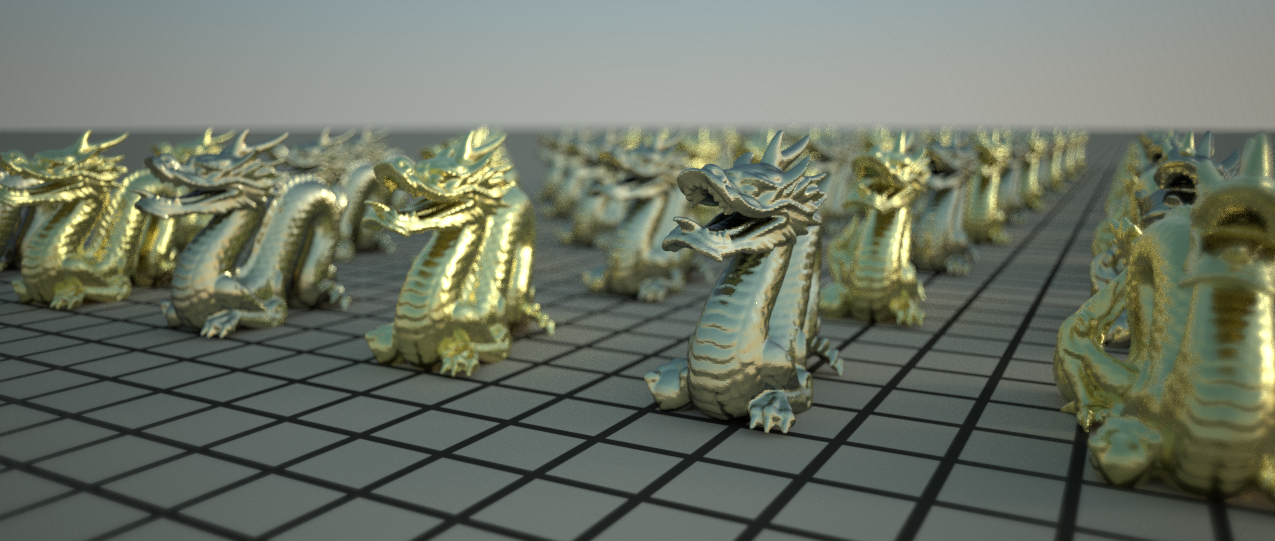

Rendering of multiple dragons. One half of the dragons has a usual gold layer as material and the other half has a multi-layered material composed from gold and a glass coating. One can clearly see the scattering in the transparent layer of the coated material.
References
-
[wenzel2014,1]
Wenzel Jakob, Eugene D'Eon, Otto Jakob, Steve Marschner "A Comprehensive Framework for Rendering Layered Materials"
ACM Transactions on Graphics (ACM SIGGRAPH 2014)
Online: http://www.cs.cornell.edu/projects/layered-sg14/
Last accessed: 18. January 2016
-
[walteretal,2]
Bruce Walter, Stephen R. Marschner, Hongsong Li, and Kenneth E. Torrance. "Microfacet Models for Refraction through Rough Surfaces"
In Proceedings of EGSR 2007
Online: https://www.cs.cornell.edu/~srm/publications/EGSR07-btdf.html
Last accessed: 18. January 2016
-
[pbrt,3]
Matt Pharr, Greg Humphreys "Physically Based Rendering, Second Edition: From Theory To Implementation"