Asteroidfield Simulation

Overview

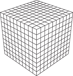
To achieve the objective of having a real time n-body engine with collision detection, we are going to use a few libraries to not reinvent the wheel. Starting with the render engine openSceneGraph [ 1], which we are using to visualize our simulation. This is a reasonable trade of due to the objective is to create the simulation engine and not to learn openGL. For our arithmetic operations we rely on the fast linear algebra library Eigen [ 2], which we are using for matrix and vector operations. We included the computational geometry algorithms library (CGAL)[ 3] into our project to compute the convex hull of our models. Each rendered object in our implementation has two meshes, one detailed mesh for rendering purpose and the simpler mesh of the convex hull for simulation purpose. To not recompile our code every time we want to run a new the engine with a different set of parameters, we include the json libary [ 4]. Now we are able to define our parameters in scene json files and load them everytime we run the program. Finally, we are using boost [ 5] to read input parameters from the user.

With a high-level perspective our code has the following pipeline. The first step before entering the simulation loop is to load all the obj models, textures and bump maps specified in the scene.json and create objects with the specified physical properties like angular rotation or linear velocity. The next step is to compute the convex hull for every mesh to speed up the simulation. Now we enter the simulation loop:

            
while(true) {
    // simulate on step
    nbodyManager->simulateStep(dt, this->_spaceObjects);

    // check for collisions
    collisionManager->handleCollisions(dt, this->_spaceObjects);

}
            
            

The infinite loop consists of two steps, first simulate a single step of movement using the n body manager and afterwards use the collision manager to handle possible collision. In the next section we are going to elaborate the implementation details of the n-body manager and the collision manager.

Implementation

Basic-Setup

For seeing how to setup the project, please read the instructions and needed frameworks in our README in the code-location. We have developed with Windows and Ubuntu, for both systems the corresponding libraries are mentioned in the README.

In principal, the most important methods are commented. For most of the classes or function it is rather obvious what should be done, since we structured it granularely with the size of this project. Here is a very quick overview of the structure of our project:

• Core (main-folder): Main files with the main-entry point for the program
• Graphics: All graphic implementation. For example GJK, EPA, convex-hull, and helper functions.
• OSG: All rendering-relevant implementations for OpenSceneGraph
  • Events: Keyboard handling
  • Particles: Particle-shader for the space-ship
  • Shaders: Shaders for the bumpmap, sun-lightning
  • Visitors: Visitors needed for OSG to extract some information (vertex-list, convex-hull, ...)
• Physics: Simulation-, N-Body- and Collision-manager.
• Scene: Needed objects to create a simulation scene.

The demo-scenes can be found in the code-directory.

The paths to load the models etc is written dynamically with CMake into the config.h file. The paths point to the directory "data" in the code repository.

Once compiled, our program can be started with several parameters. These can be looked up via "asteroid_field.exe --help".

• -h [ --help ]: Help screen
• -s [ --spheres ] arg (=10): Spheres
• -a [ --asteroids ] arg (=0): Asteroids
• -e [ --emitter ] arg (=sphere): Emitter
• -r [ --rand ] arg (=1): Random
• -g [ --gameplay ] arg (=0): Gameplay
• -f [ --saveFrames ] arg (=0): Save frame sto image files
• -j [ --sceneJson ] arg: Json file containing the scene

N-Body manager

To be able to simulate movement in space we need to implement Newtons first law of gravity, which gives us pairwise forces between two masses. $$ \vec{F} = G \cdot \frac{m_1 \cdot m_1}{|\vec{r}|^3} \vec{r} $$ where \(m_1\) and \(m_2\) are the masses and \(\vec{r}\) is the distance between the centroid of the objects: G is the gravitational constant \(6.67408 \times 10^{-11} \). Combined with the famous second law \(F = ma\) we can set up the following algorithm:

            
                # compute the forces
                for each object i:
                    for each object j, i != j:
                        vector d = distance(i.getCentroid, j.getCentorid) 
                        vector r = d.norm() * d.norm()
                        f = (G * i.getMass() * j.getMass()) / (r);
                        i.addForces(f)

                # update the physical attributes
                for each object i:
                    vector a = i.getForce() / i.getMass();
                    vector v =i.getLinearVelocity() + (dt * a);
                    i.setLinearVelocity(v);

                    vector dtv = dt * v;
                    vector p = i.getPosition() + dtv;

                    i.setPosition(p)
            
            

Accelerations

The easy and naive way uses a \(O(n^2)\) runtime. For smaller scenes this might suit absolutely and will effect the running time not significantly, but the result is still more accurate. However, for many objects, this might become a problem. Therefore we tried out two different acceleration-methods:

• We used Open-MP for parallel-loops in C++: This already significantly improved the running speed (by a factor of 4), even thought it is still \(O(n^2)\)
• A uniform spatial grid is generated (3 times as big as the scene => improvement could be to let the user define it in the scene). Then in the first step, for each object it's radius of affect is used to decide with a threshold how many neighboring cells are affected. During simulation time, the cells are updated with a list of which objects are affecting this cell. In this way, only the objects with a high enough influence are used for the calculations. The runtime for this case is \(O(n + k)\), with \(n\) being the number of objects and \(k\) being the number of influencers in the cells.

Collision manager

The collision detection consists of 3 main phases. The broad phase, the narrow phase and the collision response.

Broad phase (prune and sweep algorithm)

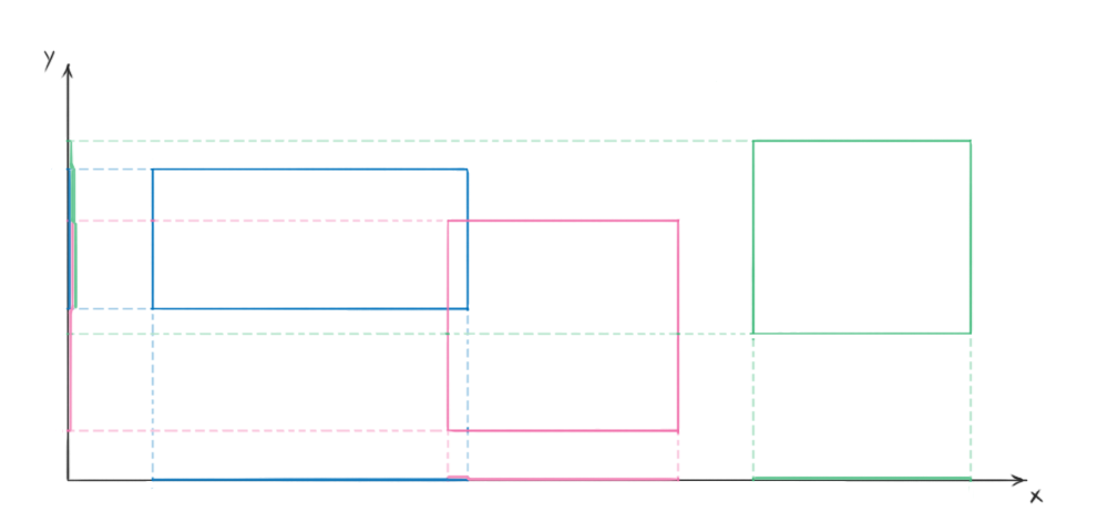
The first phase implements the prune and sweep algorithm, which objective it is to reduce number of number of computational expensive narrow collision checks. We start by computing a axis aligned bounding box for each model we are simulating. This can be done is quite fast and the check for intersection is also easy to implement. Now we are sorting the element intervals for each axis x,y and z and check if there are overlaps of object intervals. If there is an overlap in all 3 axis we know that the two AABB are intersecting and we can continue with the narrow phase checks. Due to the fact that we are storing the lists for each axis and exploiting temporal coherence the resorting can be done in a few computational steps. Since it is unlikely that the objects move significatly between two steps. (Quick sidenote: first, we defined all heavy scenes on the XY-plane, resulting to have this algorithm in the worst time complexity of \(O(n^2)\), because on z-axis each object is a possible collision with each other. Without hierarchically solving this, we simply rotated the scenes to be not aligned with an axis)

Narrow phase (GJK and EPA)

For the narrow phase in the collision detection, we implemented the GJK (Gilbert–Johnson–Keerthi distance algorithm) algorithm with the EPA (Expanding Polytope Algorithm). GJK is used to build up iteratively the Minkowski-sum, without the need to calculate the whole. In the first draft we've been using the Minkowski-sum from CGAL, which is calculating the whole sum. This resulted in a drastically bad runtime. We could significantly reduce the runtime by the iterative implementation, since this algorithm is being said to be with a constant running time. A good property of the algorithm is that

The steps for the GJK are basically the same as on the course slides.

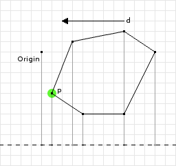
• Initialize a random direction: get the furthest point from one convex-hull and from the other the furthest in the opposite direction
• Repeat until convergence
  • Update the simplex with max 4 points
  • Check if the origin is included or max-iteration steps are passed => stop with collision by starting EPA
  • Search next point on support-function with directions to the origin.

When GJK has detected a collision, EPA needs to be run to find the correct intersection vector. Because EPA works now on a real polytope instead of only a simplex, we need to convert this first. In the normal case, our simplex has four points. In this case it can be easily created a tetrahedron with the four faces and the correct orientation of the normal.

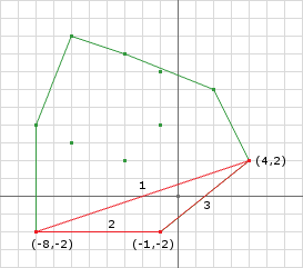
The EPA is used to find the corresponding intersection vector between the objects. This will be used later for calculating the correct collision-response. Following the steps for the EPA, which starts with the simplex found during the GJK:

• Repeat until convergence
  • Get closest face to the origin
  • Get the support-function into the direction of the faces normal
  • Expand the polytope with point from support-function and remove redundant faces
  • If the expansion is below a given threshold or the point has already been added, it converged and can go to the final step
• Calculate the intersection point on each object with the barycentric point from the intersecton-polytype

For expanding the polytope with a new support-point, following steps need to be done in order to still have a convex polytope:

• Detect each face which can be "seen" from the point
• Remove each of those faces, but remember the removed edges. Only if an edge is removed twice, it will not be contained in the new polytope. If it is removed only once, it is on the boarder of the removed faces.
• With the remaining boarders (which have removed exactly once) and the added point, all new faces can be generated

At the end, we have the global intersection vector, which can be further processed when calculating the collision-response.

Collision-response

Narrow phase creates a collision object with the colliding objects, intersection points, contact normal and a intersection vector. This is all data that we need to calculate collision response for arbitrary geometry. First, we must calculate impact speed of the colliding points on the bodies. It is the sum of four different velocities projected to the contact normal:

• First body's linear velocity
• Second body's linear velocity
• Velocity of first body's intersection point due to rotation
• Velocity of second body's intersection point due to rotation

We use this speed to calculate outgoing velocity, which is usually only a fraction of it (coefficient of restitution). We also record velocities perpendicular to the contact normal. They will be important later when we add friction.

Considering that we know the needed difference in velocities that we want to attain, we can estimate the change in linear and angular velocities of bodies. For that we calculate the moment of inertia in global frame for both bodies. By combining this with the distance of contact points from the centroid point, we determine how easy the body is to rotate. We can combine this with masses (which determine linear inertness - how easy bodies are to move), to calculate total response per unit of impulse. Because we know the difference in velocities, we can calculate the total change of impulse needed, and distribute it among the four components (translation and rotation of both bodies).

Friction complicates things a bit, but by recording projections of the closing velocity along the other two axes of the contact base, we can try to kill them too using a change in impulse. However, there is a limitation. Friction is a reactive force. It cannot make velocities point in the opposite direction. If we detect that case, we set the corresponding component to 0.

Now we have a change in linear and angular velocity. Linear velocity is easy to convert to actual coordinates by integration in the update step. However, for rotation, we must integrate angular velocity to obtain the change of angle in the time span, and then calculate and apply a rotation quaternion.

The last step involves intersection resolution. We must move objects apart so they don't intersect each other anymore at the end of the frame. We do that by distributing the translational and rotational movement based on objects' inertness. Objects which rotate easily will have a higher rotational response, while light objects will be moved further apart. In the end, both intersection points are moved by a length of intersection vector from each other. The only thing that objects' inertia determines is the ratio of both bodies' movement.

N-body results

In this section we are going to display our results for different parameters. We start with very simple settings and increase the number and complexity.

Circular orbit (2 bodies)

The goal of this experiment is to get a planet orbiting another planet in a circular way. Therefor we create a scene file (circularOrbit.json) with a sun (m = 20.0) and a earth (m = 0.1). The sun has zero linear an angular velocity and the earth $$ \vec{p} = \begin{pmatrix} -5.0 \\ 0 \\ 0 \end{pmatrix} \vec{lv} = \begin{pmatrix} 0.0 \\ 2.0 \\ 0 \end{pmatrix} $$

---

Elliptical orbit (2 bodies)

The goal of this experiment is to get a planet orbiting another planet in a elliptic way. Therefore we create a scene file (ellipticalOrbit.json) with a sun (m = 1000.0) and a earth (m = 0.1). The sun has zero linear an angular velocity and the earth $$ \vec{p} = \begin{pmatrix} -5.0 \\ 0 \\ 0 \end{pmatrix} \vec{lv} = \begin{pmatrix} 0.0 \\ 16.7299316 \\ 0 \end{pmatrix} $$

---

Figure eight (3 bodies)

The goal of this experiment is test stable 3 body configuration. Therefor we create a scene file (figureEight.json) with three planets each having a mass of one and the following positions and velocities. $$ \vec{p_1} = \begin{pmatrix} -1.0 \\ 0 \\ 0 \end{pmatrix} \vec{p_2} = \begin{pmatrix} 1.0 \\ 0 \\ 1.0 \end{pmatrix} \vec{p_3} = \begin{pmatrix} 1.0 \\ 0 \\ 0 \end{pmatrix} \vec{lv_1} = \begin{pmatrix} 0.347111 \\ 0.532728 \\ 0 \end{pmatrix} \vec{lv_2} = \begin{pmatrix} 0.347111 \\ 0.532728 \\ 0 \end{pmatrix} \vec{lv_3} = \begin{pmatrix} -0.694222 \\ -1.065456 \\ 0 \end{pmatrix} $$

---